In this blog post, we’ll give to the avid P-ADA-wan an overview of the paper Tesco Grocery 1.0, a large-scale dataset of grocery purchases in London. This paper was made by some experimented Jedi that used this dataset wisely. We tried to follow their path by extending the paper, as explained in the other blog posts.

Credits

As young Jedi, we would firstly like to thank the author of this paper, Lucas Maria Aiello, Daniele Quercia, Rossano Schifanella and Lucia Del Prete for their work on this paper.

We would also like to thank the Data Science Lab of EPFL, as this project is part of the Fall 2020 Applied Data Analysis course.

Introduction

The Tesco Grocery 1.0 dataset is a record of over 420 M food items, purchased by 1.6M fidelity card owners across Greater London. The authors aggregated the data at different levels, using the same geographical delimitations as the Office for National statistics, dividing into different granularities: LSOA (Lower Super Output Area), MSOA (Medium Super Output Area), Ward, and borough. They computed the average food product for each areas, and linked it to health outcomes strongly linked to food consumption dataset. Then, they established a correlation between the food consumed and the prevalence of health diseases in an area.

Data aggregation

We can divide the aggregation of the Tesco dataset in two main parts.

A link between the product and its nutrition properties

The first aggregation scheme happened for each of the 420 M food items entry. Each entry was under the form {customer area, GTIN, timestamp}. The GTIN (Global Trade Item Number) is used by companies to uniquely identify their trade items globally. The authors joined each entry with its corresponding nutrition informations, such as {total energy, net weight, fats, saturated fats, carbohydrates, free sugars, proteins, fibers}, on top of volume and relative volume of alcohol for drinks.

Then, they computed different data related to the nutrients informations, such as the total energy in kilocalories (kcal), as the dataset provides the amount of nutrients in grams (g). As each nutrients has a fix g / kcal ratio, the authors were able to compute the total amount of energy, as well as the relative amount of energy related to each nutrients.

On top of this, each food item is associated to one category. The categorization includes 17 non-overlapping classes, available in the Appendices.

An aggregation between food purchase and geographical areas

The authors mapped the purchases to geographical areas, as mentionned in the introduction. This aggregation scheme happened for all geographical levels, from LSOA to Borough. This aggregation scheme allowed the authors to have multiple granularity levels, which enable a wider range of studies that might benefit from having either a high number of smaller areas containing fewer datapoints or a lower number of areas characterized by more robust statistics.

Those areas have basic census statistics collected by the ONS in 2015. An exhaustive list of these statistics present in the joined dataset is available in the Appendices. The authors aggregated the Tesco data relative to each areas, and provided 3 different sets of variables.

The first group of variables expresses the Tesco penetration in an area. The representativeness, which is the ratio between the number of customers in an area and the population, is computed. A normalized representativeness is also computed.

Then, the authors decided to compute the average product bought for each area. They computed multiple nutrional properties about this average product, such as the weight or the volume, the energy, the energy - density, and the grams of each indivdual nutrients $nutrients_{i}$. Then, they compute the energy per nutrient, as well as the frequency of each nutrients, and the frequency of energey per nutrient. They managed to compute the entropy of these 2 frequencies.

The last group of variables is about the Product categories. The authors computed the probability distribution of items belonging to the 17 different product categories being purchased in area a and the entropy of that distribution. They also computed the relative weight of products belonging to any category compared to the total weight, and its entropy.

Data biases and limitations

Several limitations were pointed by the authors:

• Representativeness: As this study collect the grocery purchases from Tesco’s customers owning a Clubcard submission, this set of Clubcard owners might not be representative of the overall population.
• Coverage: The concentration of Tesco is higher in the northern part of London, thus some areas have a low penetration rate.
• Limited scope: This dataset only show the grocery purchases at Tesco - thus, the food consumption in restaurants or the food bought at other grocery stores is not included in the dataset.
• Average product As the data is aggregated to create the average product consumed in an area, this is a limitation to any study that requires an average representation at an individual level rather than at a geographical level.

Technical validation

The authors wanted to show that their aggregated dataset made sense. After a quick explanation on how to select the most representative areas, they linked their created dataset to food-related health outcomes.

Area representativeness

To ensure the representativeness of the dataset, the authors stated that we can play with the normalized representativeness in order to select the areas with the best ratio between the number of customers and the numbers of residents.

Validation of health outcomes

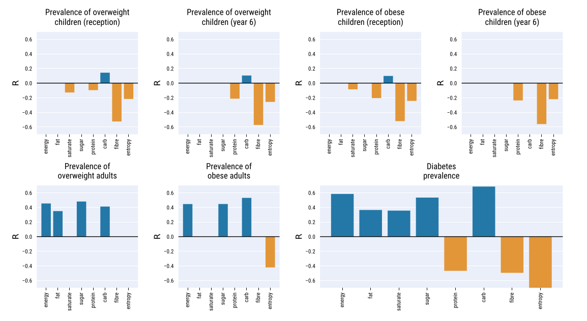
The authors joined this Tesco dataset to dataset related to obesity and Type-2 diabetes, as these health diseases are strongly correlated with diet.

The authors computed the Spearman rank correlation between the energy, the nutrients and the nutrients entropy of the average product in an area and the prevalence of obese and overweight children and adults, as well as diabetes prevalence. Those result are displayed below. We should note that only statistically significant correlations (p < 0.05) are shown.

To build stronger evidences of the link between the dataset and food related illnesses - thus, to show that the food descriptors provided dataset are not proxies, the authors then ran an ordinary least square regression.

Using the two highest-correlated factors and four control variables accounting for demographics, they managed to get a R² ratio of 0.613, which denotes a high goodness of fit. Using only the two factors energy-carbs and $H_{_energy-nutrients}$, the R² ratio remained high (0.56)

These result showed that the dataset make sense, as they found correlations which were expected between the average food product and related health diseases.

Appendices

Food categories :

fruit & vegetables; grains (e.g., bread, rice, pasta); red meat (e.g., pork, beef); poultry; fish; dairy (e.g., milk, cheese); eggs; fats & oils (e.g., butter, olive oil); sweets (e.g., chocolate, candies); readymade items (e.g., pre-cooked meal); sauces (e.g., tomato sauce, soups); tea & coffee; soft drinks (e.g., carbonated sodas); bottled water; beer; wine; spirits.

Geographical areas stastistics

population, number of males, number of females, number residents aged [0–17], number residents aged [18–64], number residents aged 65+, average age, surface area, density of residents